Overview of Simulation Graphs in Speaker Box Lite: Analyzing Speaker Performance

The Transfer Function (dB) Plot

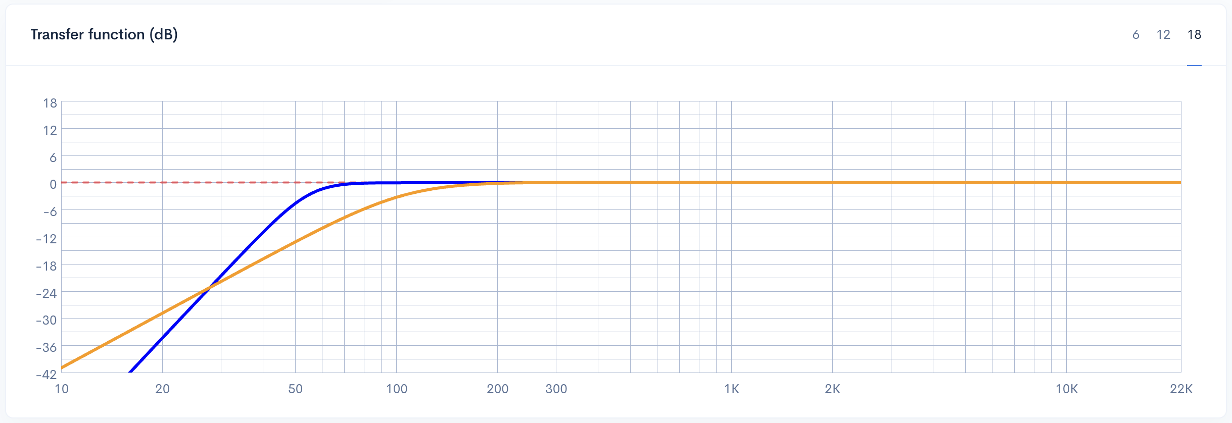
The Transfer Function plot displays the speaker's normalized frequency response, independent of input power. It focuses exclusively on how enclosure geometry and tuning influence output. The 0dB line represents the driver's nominal sensitivity - a flat response at 0dB indicates accurate signal reproduction.

The curve's "knee" marks the transition into lower bass roll-off. A critical benchmark here is the F3 point - the frequency where response drops by 3dB - which defines the system's effective low-end reach.

The roll-off slope identifies the enclosure type: sealed boxes typically feature a shallow 12dB/octave slope for a gradual transition, whereas ported designs exhibit a steeper 24dB/octave slope. While ported systems often offer deeper extension, their steeper roll-off means bass energy decreases rapidly below the tuning frequency.

Sound Pressure Level - SPL (dB) Graph

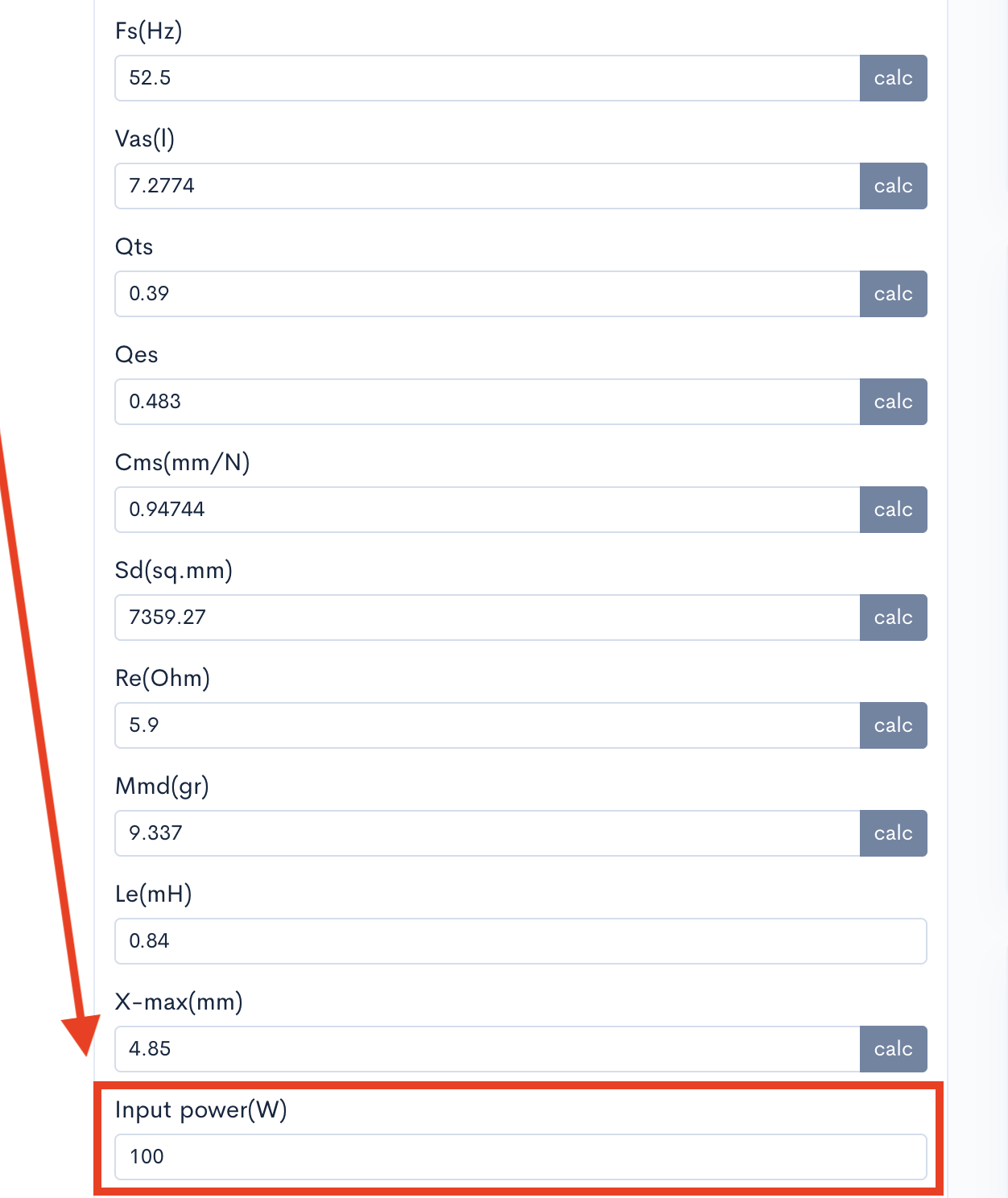
Unlike the Transfer Function, which provides a relative look at enclosure behavior, the Sound Pressure Level (SPL) graph displays the absolute output level in decibels. This plot accounts for two vital real-world variables: the driver's intrinsic sensitivity and the electrical power supplied to the voice coil. By adjusting the input power within Speaker Box Lite, you can visualize how loud the system will actually play at a standard distance - usually 1 meter.

This graph is essential for determining if a design meets your specific volume requirements. While the Transfer Function shows the shape of the bass response, the SPL graph tells you if that response is loud enough to be heard over background noise or to keep up with other components in a multi-way system. It effectively bridges the gap between theoretical enclosure performance and practical, audible results in your listening environment.

Cone Displacement (mm) and Xmax Safety

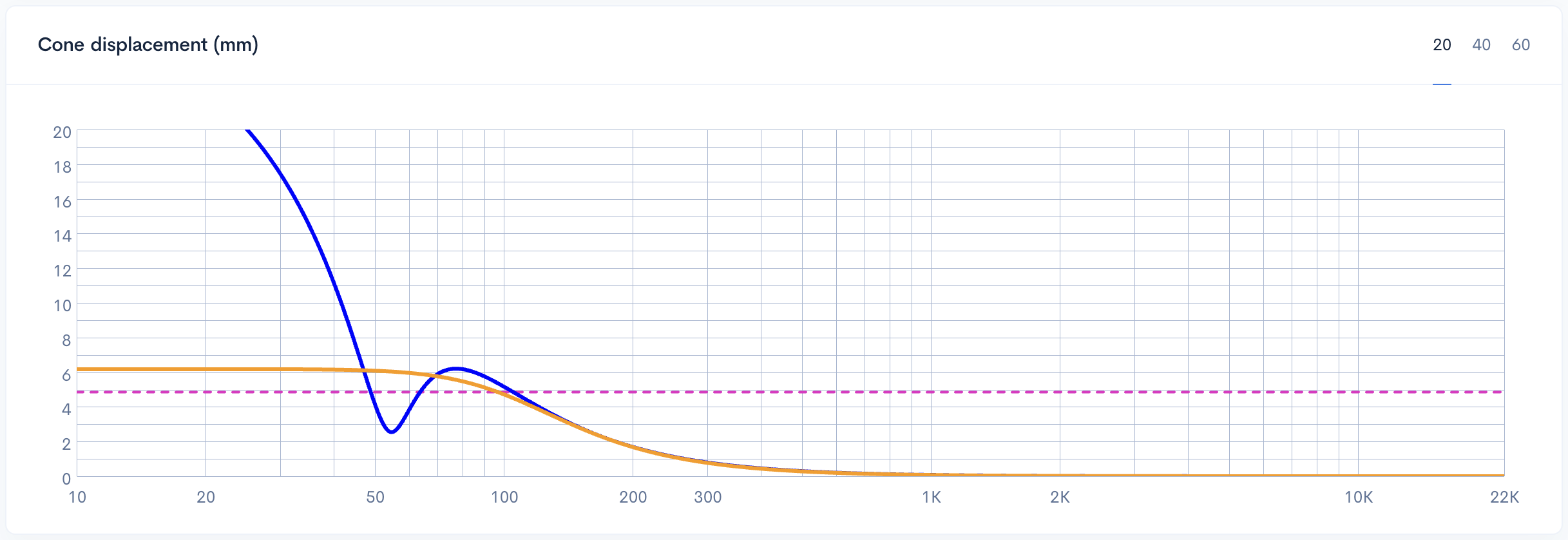
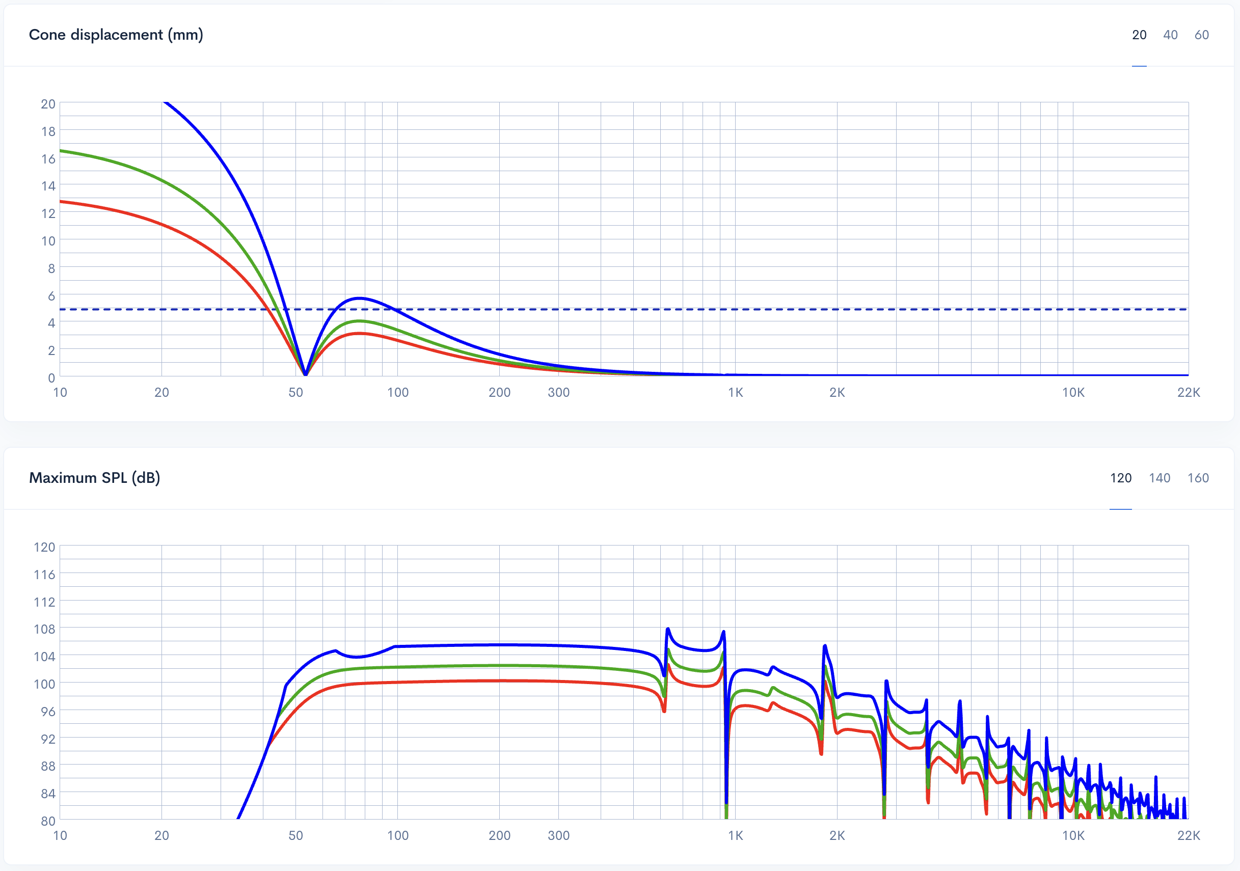
The Cone Displacement (mm) plot is essential for monitoring the physical safety of your driver. It visualizes the diaphragm's travel across the frequency spectrum relative to the input power. Within Speaker Box Lite, you will notice a horizontal line representing Xmax - the manufacturer's rated limit for linear excursion. To ensure a clean, reliable design, your displacement curve should remain below this threshold at your target wattage.

In ported enclosures, this graph reveals a characteristic dip at the tuning frequency (Fb), where the vent air provides maximum resistance and cone movement is minimized. However, below this point, the driver loses acoustic loading and displacement rises rapidly. This spike is why a subsonic filter is critical; it protects the speaker from bottoming out at frequencies the box cannot control. Monitoring this plot helps you balance output with mechanical longevity.

Maximum Power (W) and Maximum SPL (dB)

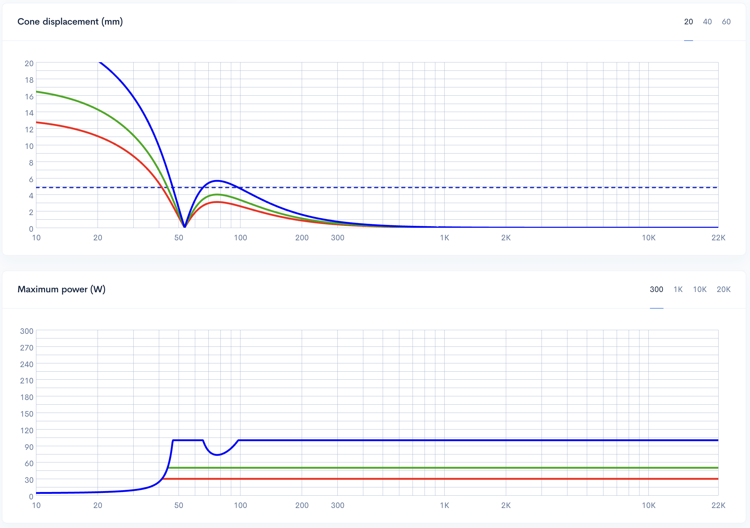
The Maximum Power (W) plot in Speaker Box Lite is a dynamic calculation that identifies the bottleneck of your speaker's performance at every frequency. It integrates two primary constraints: the driver's thermal power rating and its mechanical excursion limit - Xmax. While a speaker might be rated for 500W thermally, the graph often shows a significant drop in power handling at low frequencies where the cone reaches its physical limits much sooner. This visual data prevents the common mistake of assuming a driver can handle its full rated power across the entire spectrum.

Complementing this is the Maximum SPL (dB) graph, representing the absolute ceiling of the system's output. This plot combines box efficiency and the calculated maximum power to show the loudest possible volume the speaker can produce without damage. By analyzing this curve, designers can identify where the system might fall short of performance goals, ensuring the final build meets output requirements without risking hardware failure.

Impedance (Ohm) - Tracking Resonance

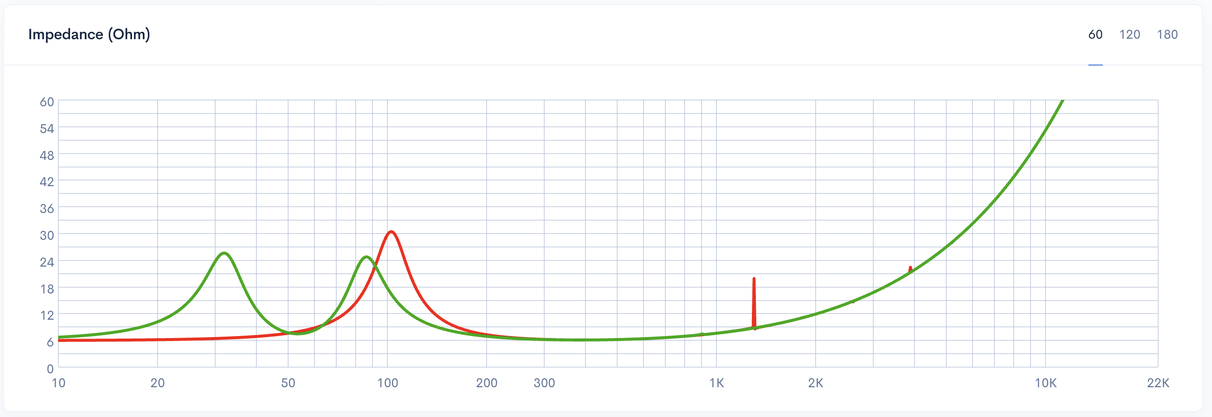
The Impedance (Ohm) graph is a critical diagnostic tool that reveals how the loudspeaker interacts electrically with the amplifier. By observing the peaks, you can pinpoint the system's resonant frequency: a single peak represents the resonance (Fc) in a sealed enclosure, while a double-peak structure identifies the tuning frequency (Fb) at the valley between them in a ported design.

This plot allows you to verify if your physical build matches the simulation. If the measured impedance peaks shift from the predicted values, it indicates discrepancies in box volume or port dimensions. Furthermore, monitoring the minimum impedance is vital for protecting your hardware, as low-impedance dips significantly increase the current load on the amplifier. This graph is also indispensable for adjusting crossovers. Since passive filters are sensitive to impedance fluctuations, knowing the exact Ohm value at the transition point ensures your crossover behaves as intended for a seamless audio response.

Vent Air Velocity (m/s) - Preventing Port Chuffing

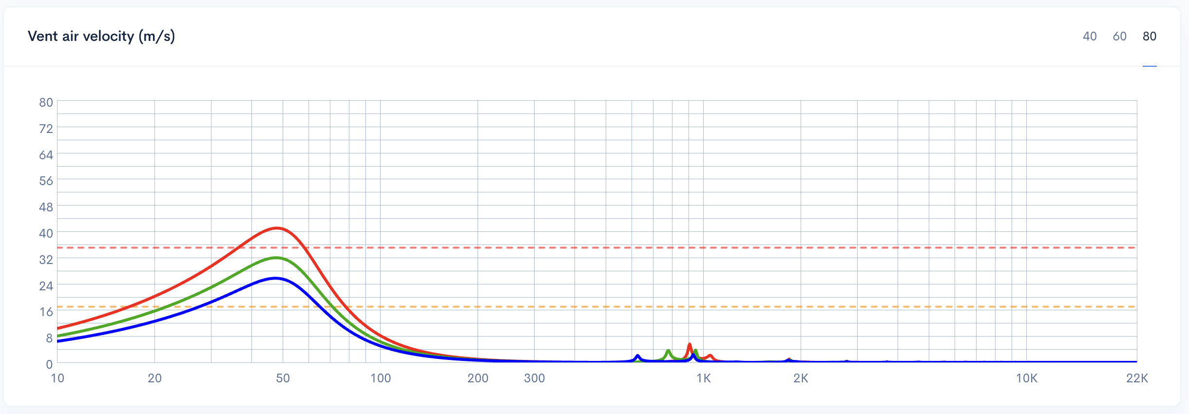
The Vent Air Velocity (m/s) graph is essential for detecting potential "chuffing" - the audible turbulence caused by air moving too fast through a port. In Speaker Box Lite, this graph includes two critical boundary lines to guide your design. Keeping your velocity below 17 m/s ensures a clean, silent port response, which is the preferred standard for high-fidelity builds. Values between 17 and 35 m/s represent a moderate range; while potentially acceptable for some applications, they risk becoming audible during high-output peaks.

Anything exceeding 35 m/s is considered very bad, leading to severe port compression and distracting noise. To optimize this, adjust the port diameter or shape within the software. Increasing the port area lowers the velocity but requires a longer vent to maintain your target tuning. If the graph shows values entering the danger zone, widening the port is the most effective way to ensure smooth airflow and maintain bass clarity.

Transfer Function Phase (°)

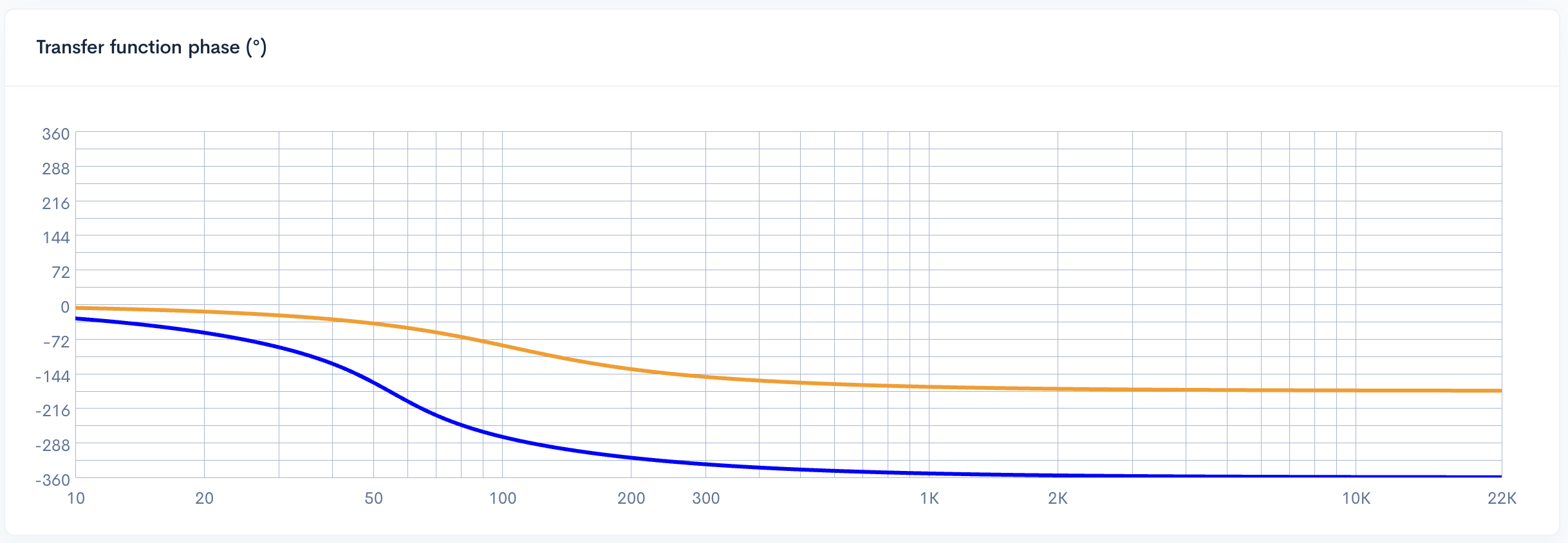
The Transfer Function Phase (°) graph illustrates how the enclosure alters the timing of the sound waves relative to the input signal across the frequency spectrum. Every speaker enclosure introduces some degree of phase shift; for instance, a standard sealed box typically results in a 180-degree shift at the low end, while a ported design exhibits a 360-degree rotation.

These shifts are directly tied to the alignment type and the steepness of the roll-off. When analyzing this plot in Speaker Box Lite, the primary goal is to look for smooth, gradual transitions. Sharp, abrupt changes in the phase curve often correspond to resonances or poor transient response, which can lead to "muddy" sound. A well-designed system maintains phase consistency, ensuring that the driver integrates seamlessly with other components and preserves the intended timing of the audio signal.

Transfer Function Group Delay (ms)

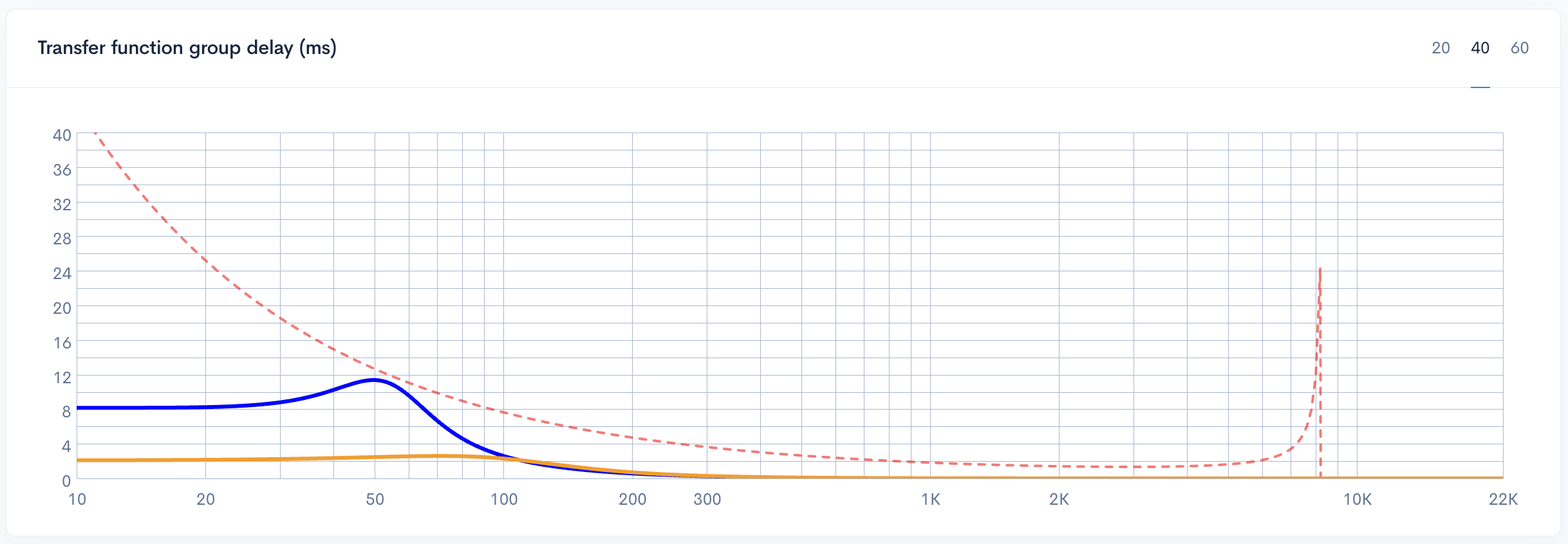
The Transfer Function Group Delay (ms) graph is a critical metric for evaluating the transient response of your enclosure design. Defined as the time it takes for a signal to pass through the system, group delay quantifies the latency introduced by the box at specific frequencies. High group delay in the lower registers is the primary culprit behind "slow" or "muddy" bass, as it indicates the driver is struggling to stop and start in sync with the input signal.

To ensure a "tight" and punchy low end, engineers typically aim for delay levels under 15-20ms at 40Hz. Speaker Box Lite simplifies this analysis by providing a recommended boundary line directly on the plot. For the best acoustic results, always strive to keep your curve below this threshold. This ensures the system responds accurately to rapid transients without the excessive energy storage that leads to poor signal integrity and a lack of definition.